Getting Started with the Snowflake Query Profile

If you struggle with slow and expensive queries on Snowflake you need to master the query profile. Learning to read a query profile will help you understand and address the bottlenecks that impact performance.

When any query is run on Snowflake, the executed SQL is translated into a streaming data pipeline. For the most part that pipeline is invisible. There's no way to interact with it, modify it, or introspect it. SQL in, results out. But when queries run for too long, the need may arise for you to look under the covers and find out what's actually taking so much time.

That's where profiling comes in. The query profile gives a peek into the Snowflake black box, providing an X-ray of your query, telling you the layout, configuration, and performance breakdown of the query's data pipeline.

To get started, pull up  profile for a query. You can find it a few ways:

• In the new Snowsight console under Activity > Query History  > {query} > Query Profile
• In the Classic console under History > {query id} > Profile
• Programmatically with the GET_QUERY_OPERATOR_STATS(...) system function.

The query profile has two main parts: a graph view of the data pipeline and a statistics panel.

The graph view lays out each step of the data pipeline as a set of operator nodes. Each box in the graph represents a single node in the pipeline. Arrows between the boxes show the flow of data between nodes. The arrows are labeled with the count of rows flowing between nodes. All together, these operator nodes represent the data pipeline for your query.

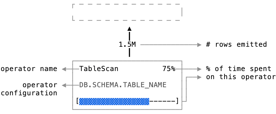
The statistics panel provides critical performance details, including:

• Total time spent
• A list of the most expensive operators
• A breakdown of time spent into high-level categories like CPU processing, network transfer, and disk I/O

Let's consider an example: imagine we need to calculate total sales by store.

SELECT
    store_id
  , COUNT(*) as num_orders
  , SUM(revenue) as total_sales

FROM store_orders

GROUP BY
    store_id

When executed, this query produces the following profile:

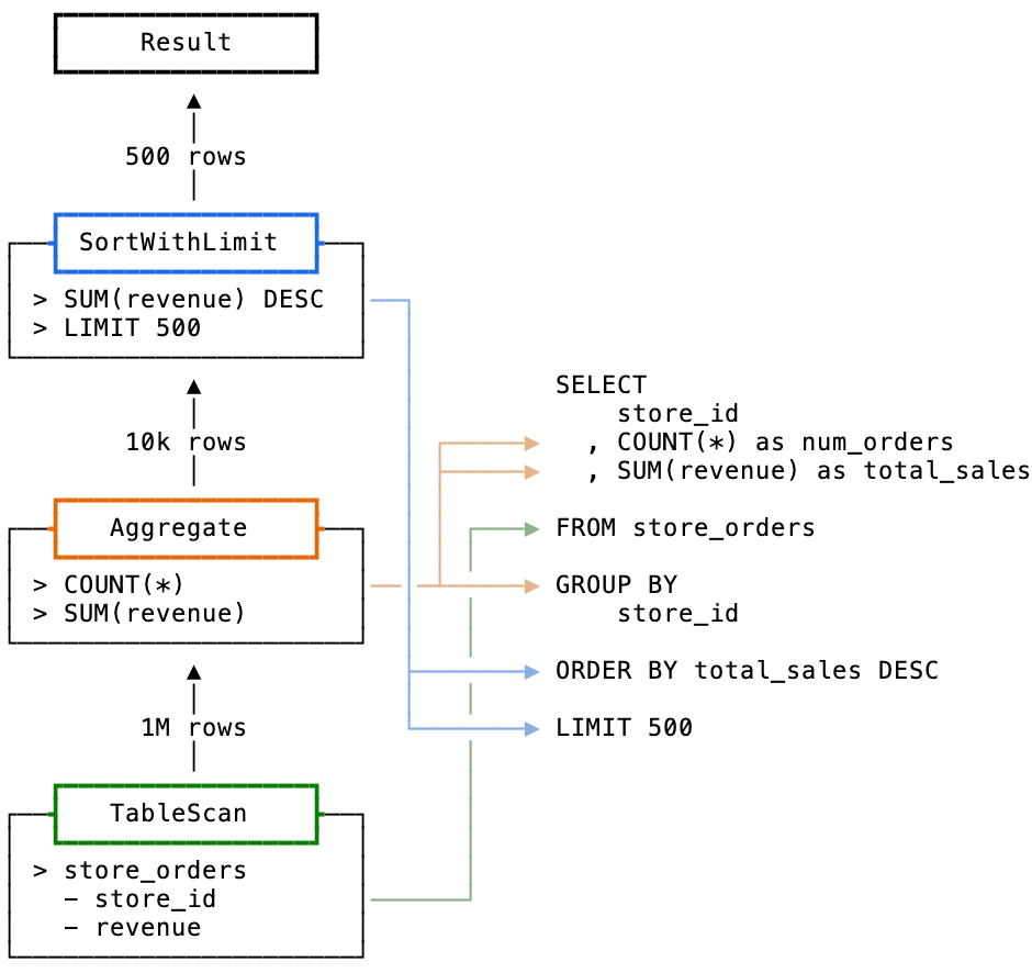
This query was translated into a data pipeline with 4 operators: Result, SortWithLimit, Aggregate, and TableScan. There are many operator types, these 4 represent a handful of the most common you will run in to in the wild. In the Snowflake UI, these steps are shown in a tree organized last-to-first: the operator on top is the final step in the pipeline, the operator on bottom is the start.

Let's review what each operator does.

TableScan

Most queries start with a TableScan operator, it is responsible for reading data from a table. This is the most important operator to know, as its used in most queries and it's easy to optimize.

A TableScan operator reads data from cloud storage and emits that data as rows. It is configured with a single table name, a set of columns, and a set of micro-partitions to scan. Typically, a pipeline will have one TableScan operator for each FROM statement in your query.

TableScans benefit from a common optimization called micro-partition pruning. This typically occurs when the query specifies a WHERE condition, telling the optimizer that only some of the table's data is required. You know that pruning has occurred when the Partitions scanned statistic of the TableScan operator is lower than Partitions total. Clustering or sorting a table on the columns frequently used in WHERE statements will improve pruning rates, making queries run faster.

Aggregate

The Aggregate operator is responsible for calculating any aggregate functions in a query. If the query specifies more than one aggregate function, those expressions get rolled up into a single operator. Its purpose is straightforward: this operator takes in a stream of rows, aggregates them according to the query, and emits the final aggregate values.

SortWithLimit

This is a special operator that combines both a Sort and Limit into one SortWithLimit operator. Its job is to sort data and return the top N items, determined by the ORDER BY and LIMIT clauses respectively. Combining Sort and Limit into one allows the data pipeline to quit sorting early, aiding performance.

Result

The simple Result operator will appear as the final step for most SELECT queries - it returns the final rows back to the client that issued the query. It also saves the result in Snowflake's result cache. This lets you fetch the results later without re-running the entire pipeline. Also, if you happen to execute the exact same query and the underlying data hasn't changed, Snowflake will skip execution completely and serve the results straight from cache.

This example query breaks down into a few straightforward operators. In the most extreme cases, complex queries will include hundreds of operator nodes.

For other kinds of operators, you can check the Snowflake documentation, which includes a list of the most common operator types. It's not exhaustive, but it covers most of what you should expect to see when reviewing profiles.

Those are the basics of Snowflake's query profile. In review, the profile includes:

• A detailed view of the data pipeline that's executed for a query
• A high-level performance overview including query statistics, performance breakdown, and a list of expensive operators
• A breakdown of each step of the pipeline as a tree of operator nodes and the relationships between those nodes
• A detailed view of each operator, with configuration and performance statistics

If you want to learn more, the Activity section of the Snowsight documentation is a good place to continue learning about the query profile.