Understanding the Snowflake Query Optimizer

Imagine you design factories.

You are preeminent in your field, a singular talent. These aren't just any factories - you design the best. Using cleverness and craft you imagine factory designs that are elegant and streamlined. No inch of space wasted, not an inefficiency in sight. But for you, that's not enough.

Imagine you want to design a megafactory - a factory that designs factories - encapsulating everything you know into one automated machine. You embark on an impossible journey. How can you anticipate every possible factory variation? How do you craft rules to convert an arbitrary factory into one that has an elegant, efficient design?

That is the plight of a query optimizer - it is the factory that creates factories. To take endlessly complicated query plans and forge them into efficient pipelines of data.

The job of a query optimizer is to reduce the cost of queries without changing what they do. Optimizers cleverly manipulate the underlying data pipelines of a query to eliminate work, pare down expensive operations, and optimally re-arrange tasks.

Query optimizers aren't unique to Snowflake, any serious database has one. The history of query optimization is deep and complicated, originating with FORTRAN and rooted in compilers.

To write efficient queries in Snowflake, there are three types of optimizations you need to know about: scan reduction, limiting the volume of data read, query rewriting, reorganizing a query to reduce cost, and join optimization, the NP-hard problem of optimally executing a join.

In this post, I'll share a reference of most common optimizations you might expect to see when working with Snowflake.

Part 1: Scan reduction

The less data used, the faster a query will be. This applies to every database ever invented.

The first step in many query plans is a table scan. Before you can aggregate or analyze, the data in a table must be read into memory. A common way to optimize a query is to limit the volume of data read, scan reduction helps achieve that.

If you've used a transactional database like Postgres or SQL Server, you may be familiar with database indexes. An index is an enhancement added to a column that speeds up queries. When an indexed column is queried, the database uses it to efficiently pre-filter data, skipping any data that isn't strictly necessary.

Unfortunately, Snowflake doesn't have indexes. They use a different set of techniques to skip unnecessary data. In part 1, I'll review strategies used by the optimizer to limit the volume of data it needs to scan.

Columnar storage

Snowflake uses a columnar storage model, making use of a CPU-cache friendly file format called PAX. Columnar storage organizes data by grouping column values together, you can think of it like a CSV turned on its side. The start and end of each each group of values is included in the file's metadata.

The benefit of this columnar approach is that Snowflake only needs to read data for the columns used in a query, it can skip all others. This is one reason why you're more likely to encounter the One Big Table data modeling pattern in columnar databases.

Partition pruning

Partition pruning is the most important optimization in Snowflake. How you load data, update tables, and materialize marts will have a direct impact on pruning. And as you will find out, many other optimizations are designed to maximize pruning, even in complex, highly-joined queries.

Tables are stored in files called partitions. Partitions are written in compressed 16MB blocks and contain a subset of a table's rows in a columnar file format.

Before a query is executed, Snowflake decides which data it needs to read (aka scan) to fulfill that incoming request. In the worst case, Snowflake reads all available files for a table, known as a full table scan. Ideally though, the optimizer takes advantage of partition metadata to decide which data it can skip, in a process called partition pruning. Pruning just means skipping files.

Without indexes, Snowflake relies on the sort order of your data to perform pruning. Like an index, if your table is well sorted on a column, the optimizer can use pruning to skip unnecessary data and speed query execution time.

Snowflake maintains accurate metadata on each partition that makes up a table. Total statistics like row count and size in bytes are tracked for the table and each partition. Within each partition, the min/max values, null count, and distinct count of each column are tracked.

This example demonstrates how pruning works. The incoming user query has a filter on order_date. During the optimization step, the table's metadata is checked to determine which partitions are necessary and which can be skipped.

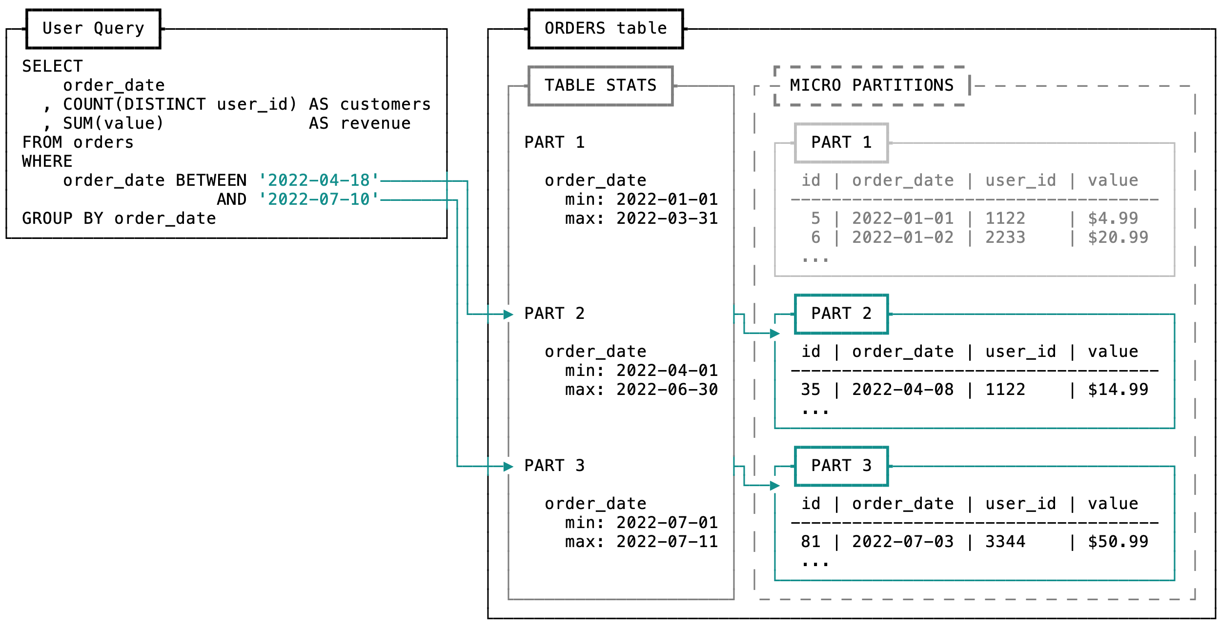
Table scan elimination

What's the fastest way to scan a table? Not scanning it at all!

Similar to partition pruning, Snowflake will check to see if it's even necessary to read a table at all. If a table is referenced but not needed, Snowflake will skip scanning the table entirely.

Data compression

Snowflake compresses all data by default, dynamically choosing a compression algorithm for each column in a partition.

Since compression is applied within partition files, tables benefit from densely packed partitions. The more rows in a partition, the better. Many standard data types benefit from compression, but be wary of hard-to-compress data like UUIDs, hashes, and semi-structured data (JSON) as they can increase scan times.

Part 2: Query rewriting

You thought your query told Snowflake what to do. You were wrong.

As a part of execution, a query is parsed into a query plan - the set of steps required to perform the computation. The job of the optimizer is to rewrite that query plan to a lower cost but logically equivalent one.

In data-intensive systems, this is called logical optimization. This is a complicated topic which includes far too many optimizations to cover here. If you're interested to learn more, I recommend reading about Spark's Catalyst optimizer which implements many of the same techniques as Snowflake.

In part 2, I'll review a few key ways that Snowflake rewrites queries to help them run faster.

Table replacement

Like a pharmacist handing out generic medication, the optimizer can replace the table you asked for with a lower cost alternative.

If you've created a materialized view using a table, Snowflake will use that instead if it's logically equivalent and cheaper to query.

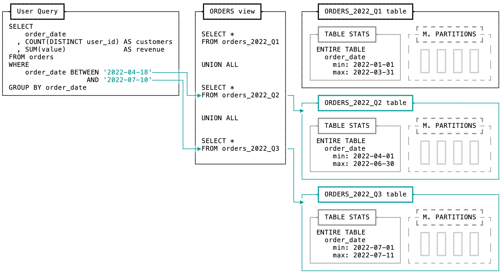
Snowflake will also use metadata to replace tables. The optimizer checks a query for statements that can be served directly from metadata, skipping a potential table scan.

In this example, the subquery to check the maximum value of order_at is replaced with a constant value, eliminating the order_fact entirely. This is a pattern commonly used in dbt for incremental materialization.

-- Before

SELECT *
FROM orders_raw
WHERE
    order_at >= ( SELECT MAX(order_at) FROM orders_fact )
                         ^^^^^^^^^^^^^

-- After

SELECT *
FROM orders_raw
WHERE
    order_at >= '2022-09-01 01:59:59'::DATETIME
                            

Constant inlining

Also called constant folding, Snowflake will take any constants, variables, or literal expressions and propagate that fixed value throughout your query. This optimization pairs well with lateral column aliases - using a column aliased earlier in the same SELECT - allowing you to compose more interpretable business logic SQL.

-- Before

SELECT 
    user_id
  , total_spend
  , 50 AS low_spend_threshold
  , (total_spend <= low_spend_threshold) AS is_low_spender
                    ^^^^^^^^^^^^^^^^^^^
FROM users

-- After

SELECT 
    user_id
  , total_spend
  , 50 AS low_spend_threshold
  , (total_spend <= 50) AS is_low_spender
FROM users
                            

Function inlining

Similar to constant inlining, Snowflake will replace some function calls with the equivalent implementation. This lets you confidently practice Dont Repeat Yourself principles without having to worry about performance impact.

If you write your own user-defined functions (UDFs), it's important to note that Snowflake will only perform inlining on SQL language functions. SQL UDFs are executed in the core engine, whereas UDFs in Java, Javascript, and Python are run in a separate execution environment. That separate environment means they can't be inlined.

CREATE FUNCTION discount_rate(paid, retail_price)
AS
SELECT 1 - (paid / retail_price)
;

-- Before

SELECT
    order_id
  , discount_rate(order_value, total_sku_price) as discount_rate_pct
    ^^^^^^^^^^^^^
FROM orders

-- After

SELECT
    order_id
  , 1 - (order_value / total_sku_price) as discount_rate_pct
FROM orders
                            

Lazy evaluation

Analytical queries often perform column transformations that are expensive, like using a regular expression to extract data from unstructured text. The optimizer defers these transformations to as late as possible in query execution. This lets filters run first, reducing the total dataset before expensive functions get executed. This is called lazy evaluation, and impacts both built-in and user-defined function calls.

The VOLATILE/IMMUTABLE keywords for UDFs are similar in spirit to lazy evaluation. If a UDF is guaranteed to return the same output for identical input, you should mark it as IMMUTABLE. This tells Snowflake it can cache the result of a function call, further reducing how often it gets executed.

-- Before

SELECT
    order_id
  , parse_geolocation(address) as geolocation
    ^^^^^^^^^^^^^^^^^
FROM orders
WHERE
    is_cancelled = TRUE

-- After

WITH cancelled_orders AS (
  SELECT
      order_id
    , address
  FROM orders
  WHERE
      is_cancelled = TRUE
)
  
SELECT
    order_id
  , parse_geolocation(address) as geolocation
FROM cancelled_orders
                            

Column pruning

Column pruning eliminates columns that are referenced but unused in a query.

This example demonstrates how column pruning can be useful. Even though the query specifies a SELECT *, only 2 columns end up being used. The optimizer recognizes this and eliminates the rest of the columns from the query plan.

-- Before

WITH users AS (
  SELECT *
  ^^^^^^^^
  FROM users_raw
)

SELECT
    user_id
FROM users
WHERE
    account_type = 'paid'

-- After

WITH users AS (
  SELECT
      user_id
    , account_type
  FROM users_raw
)

SELECT
    user_id
FROM users
WHERE
    account_type = 'paid'

Predicate pushdown

filtering data earlier helps reduce cost. In predicate pushdown, the optimizer looks for predicates - filtering expressions in WHERE and HAVING clauses. It moves these expression as early in the query as possible, pushing them "down" in the query plan's execution tree.

-- Before

WITH orders AS (
  SELECT *
  FROM orders_raw
)
  
SELECT
    SUM(order_value) AS last_month_revenue
FROM orders
WHERE
    order_date BETWEEN '2022-08-01' AND '2022-08-31'
    ^^^^^^^^^^

-- After

WITH orders AS (
  SELECT *
  FROM orders_raw
  WHERE
      order_date BETWEEN '2022-08-01' AND '2022-08-31'
)
  
SELECT
    SUM(order_value) AS last_month_revenue
FROM orders
 

Part 3: Join optimization

The art and science of how to execute a join is an active area of research in computer science. Just at SIGMOD 2022 alone you can find several research papers working on the join problem.

The majority of join optimizations in Snowflake are under the hood, like dynamically selecting a join strategy or building bloom filters. In part 3, I'll review a handful of the more visible join optimizations you may discover in the wild.

Join filtering

Joins are expensive, reducing data volume on both sides of a join is critical. For joins, the optimizer performs a special form of predicate pushdown called join filtering.

When join filtering is active, it's visible in the query profile as a JoinFilter operator node. This node uses query predicates, table metadata, and other logic to pre-filter data before it gets passed to a join.

Transitive predicate generation

This optimization is closely related to join filtering and predicate pushdown, with one unique exception: it creates new predicates, instead of moving around existing ones.

If you join tables together and filter one table on the join column, the optimizer will mirror this filter to the other table. This generates a new predicate, ensuring both tables are filtered to the same set of data before they're joined.

-- Before

SELECT *
FROM (
        SELECT *
        FROM website_traffic_by_day
        WHERE traffic_date >= '2022-09-01'
              ^^^^^^^^^^^^
     ) AS traffic
LEFT JOIN revenue_by_day AS revenue
  ON traffic.traffic_date = revenue.order_date

-- After

SELECT *
FROM (
        SELECT *
        FROM website_traffic_by_day
        WHERE traffic_date >= '2022-09-01'
     ) AS traffic

LEFT JOIN (
        SELECT *
        FROM revenue_by_day
        WHERE order_date >= '2022-09-01'
     ) AS revenue

  ON traffic.traffic_date = revenue.order_date

Predicate ordering

When executing a join, Snowflake needs to check if all join conditions match. When a query specifies multiple join conditions, the optimizer re-orders the conditions from most selective to least selective.

In this example, there are many rows in both tables that match the category predicate making this join condition less selective, it doesn't filter many rows. The date predicate is more selective because relatively fewer rows match between the two tables. The optimizer will re-arrange these conditions, swapping from the original order.

-- Before

SELECT
FROM inventory
JOIN products
  ON inventory.category = products.category
     ^^^^^^^^^^^^^^^^^^^^^^^^^^^^^^^^^^^^^^
 AND inventory.stock_date = products.first_active_date
  
-- After

SELECT
FROM inventory
JOIN products
  ON inventory.stock_date = products.first_active_date
 AND inventory.category = products.category

Join elimination

This is a new feature in Snowflake that takes advantage of foreign key constraints. In a way, this is the first optimizer hint in Snowflake.

When two tables are joined on a column, you have the option to annotate those columns with primary & foreign key constraints using the RELY property. Setting this property tells the optimizer to check the relationship between the tables during query planning. If the join isn't needed, it will be removed entirely.

You've just learned about the most important optimizations used by Snowflake to execute query plans efficiently. If you made it this far, you're an optimization pro.

Learning more

If you want to learn more about databases and query optimization, I highly recommend these resources.

Mahdi Yusuf's Architecture Notes, including Things You Should Know About Databases.

The Quarantine Database Tech Talks series hosted by Carnegie Mellon. Most of my knowledge of the Snowflake query optimizer comes from Jiaqi Yan's talk.

Jaime Brandon's blog Scattered Thoughts, including How Materialize and other databases optimize SQL subqueries.

Justin Jaffray's self-titled blog, including Understanding Cost Models.